Explained variation

In statistics, explained variation or explained randomness measures the proportion to which a mathematical model accounts for the variation (= apparent randomness) of a given data set. Often, variation is quantified as variance; then, the more specific term explained variance can be used.

The complementary part of the total variation/randomness/variance is called unexplained or residual.

The simplified assumption of explained variance as equal to the square of the correlation coefficient has been criticized. "for most social scientists, is of doubtful meaning but great rhetorical value".^[1]^[2]

1 Definition
- 1.1 Information gain by better modelling
- 1.2 Information gain by a conditional model
2 Special cases and generalized usage
3 Criticism
4 Notes
5 Further reading
6 External links

Definition

Explained variation is a relatively recent concept. The most authoritative source seems to be Kent (1983) who founded his definition on information theory.

Information gain by better modelling

Following Kent (1983), we use the Fraser information (Fraser 1965)

$F(\theta) = \int \textrm{d}r\,g(r)\,\ln f(r;\theta)$

where $\textrm{d}r\,g(r)$ is the probability density of a random variable $R\,$ , and $f(r;\theta)\,$ with $\theta\in\Theta_i$ ( $i=0,1\,$ ) are two families of parametric models. Model family 0 is the simpler one, with a restricted parameter space $\Theta_0\subset\Theta_1$ .

Parameters are determined by maximum likelihood estimation,

$\theta_i = \mbox{arg max}_{\theta\in\Theta_i} F(\theta)$ .

The information gain of model 1 over model 0 is written as

$\Gamma(\theta_1:\theta_0) = 2 [ F(\theta_1)-F(\theta_0) ]\,$

where a factor of 2 is included for convenience. Γ is always nonnegative; it measures the extent to which the best model of family 1 is better than the best model of family 0 in explaining g(r).

Information gain by a conditional model

Assume a two-dimensional random variable $R=(X,Y)$ where X shall be considered as an explanatory variable, and Y as a dependent variable. Models of family 1 "explain" Y in terms of X,

$f(y|x;\theta)$ ,

whereas in family 0, X and Y are assumed to be independent. We define the randomness of Y by $D(Y)=\exp[-2F(\theta_0)]$ , and the randomness of Y, given X, by $D(Y|X)=\exp[-2F(\theta_1)]$ . Then,

$\rho_C^2 = 1-D(Y|X)/D(Y)$

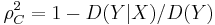
can be interpreted as proportion of the randomness which is explained by X.

Special cases and generalized usage

For special models, the above definition yields particularly appealing results. Regrettably, these simplified definitions of explained variance are used even in situations where the underlying assumptions do not hold.

Linear regression

The fraction of variance unexplained is an established concept in the context of linear regression. The usual definition of the coefficient of determination seems to be compatible with the fundamental definition of explained variance.

Correlation coefficient as measure of explained variance

Let X be a random vector, and Y a random variable that is modeled by a normal distribution with centre $\mu%2B\Psi^\textrm{T}X$ . In this case, the above-derived proportion of randomness $\rho_C^2$ equals the squared correlation coefficient $R^2$ .

Note the strong model assumptions: the centre of the Y distribution must be a linear function of X, and for any given x, the Y distribution must be normal. In other situations, it is generally not justified to interpret $R^2$ as proportion of explained variance.

Explained variance in principal component analysis

"Explained variance" is routinely used in principal component analysis. The relation to the Fraser-Kent information gain remains to be clarified.

Criticism

As "explained variance" essentially equals the correlation coefficient $R^2$ , it shares all the disadvantages of the latter: it reflects not only the quality of the regression, but also the distribution of the independent (conditioning) variables.

In the words of one critic: "Thus $R^2$ gives the 'percentage of variance explained' by the regression, an expression that, for most social scientists, is of doubtful meaning but great rhetorical value. If this number is large, the regression gives a good fit, and there is little point in searching for additional variables. Other regression equations on different data sets are said to be less satisfactory or less powerful if their $R^2$ is lower. Nothing about $R^2$ supports these claims".^[3] And, after constructing an example where $R^2$ is enhanced just by jointly considering data from two different populations: "'Explained variance' explains nothing" ^[4]^[5]

Notes

^ Achen 1990, p. 183
^ C H Achen (1982)
^ Achen 1982, p. 58
^ Achen 1990, p. 183
^ C H Achen (1982)